SQL is one of the major tools of data analysis. It provides filtering, transforming and aggregation functionalities, and we can use it to process big volume of data with the help of Hive and Hadoop. However, legacy SQL does not support operations like grouped ranking and moving average, because the GROUP BY clause can only produce one aggregation result for each group, but not for each row. Fortunately, with the new SQL standard coming, we can use the WINDOW clause to compute aggregations on a set of rows and return the result for each row.
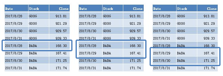
For instance, if we want to calculate the two-day moving average for each stock, we can write the following query:
1 | SELECT |
OVER, WINDOW and ROWS BETWEEN AND are all newly added SQL keywords to support windowing operations. In this query, PARTITION BY and ORDER BY works like GROUP BY and ORDER BY after the WHERE clause, except it doesn’t collapse the rows, but only divides them into non-overlapping partitions to work on. ROWS BETWEEN AND here constructs a window frame. In this case, each frame contains the previous row and current row. We’ll discuss more on frames later. Finally, AVG is a window function that computes results on each frame. Note that WINDOW clause can also be directly appended to window function:
1 | SELECT AVG(`close`) OVER (PARTITION BY `stock`) AS `mavg` FROM `t_stock`; |
Window Query Concepts
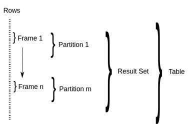
SQL window query introduces three concepts, namely window partition, window frame and window function.
PARTITION clause divides result set into window partitions by one or more columns, and the rows within can be optionally sorted by one or more columns. If there’s not PARTITION BY, the entire result set is treated as a single partition; if there’s not ORDER BY, window frames cannot be defined, and all rows within the partition constitutes a single frame.
Window frame selects rows from partition for window function to work on. There’re two ways of defining frame in Hive, ROWS AND RANGE. For both types, we define the upper bound and lower bound. For instance, ROWS BETWEEN UNBOUNDED PRECEDING AND CURRENT ROW selects rows from the beginning of the partition to the current row; SUM(close) RANGE BETWEEN 100 PRECEDING AND 200 FOLLOWING selects rows by the distance from the current row’s value. Say current close is 200, and this frame will includes rows whose close values range from 100 to 400, within the partition. All possible combinations of frame definitions are listed as follows, and the default definition is RANGE BETWEEN UNBOUNDED PRECEDING AND CURRENT ROW.
1 | (ROWS | RANGE) BETWEEN (UNBOUNDED | [num]) PRECEDING AND ([num] PRECEDING | CURRENT ROW | (UNBOUNDED | [num]) FOLLOWING) |
All window functions compute results on the current frame. Hive supports the following functions:
FIRST_VALUE(col),LAST_VALUE(col)returns the column value of first / last row within the frame;LEAD(col, n),LAG(col, n)returns the column value of n-th row before / after current row;RANK(),ROW_NUMBER()assigns a sequence of the current row within the frame. The difference isRANK()will contain duplicate if there’re identical values.COUNT(),SUM(col),MIN(col)works as usual.
Hive Query Examples
Top K
First, let’s create some test data of employee incomes in Hive:
1 | CREATE TABLE t_employee (id INT, emp_name VARCHAR(20), dep_name VARCHAR(20), |
We can use the RANK() function to find out who earns the most within each department:
1 | SELECT dep_name, emp_name, salary |
Normally when there’s duplicates, RANK() returns the same value for each row and skip the next sequence number. Use DENSE_RANK() if you want consecutive ranks.
Cumulative Distribution
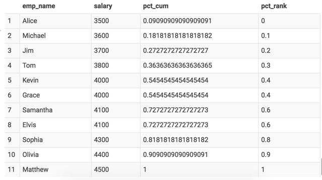
We can calculate the cumulative distribution of salaries among all departments. For example, salary 4000‘s cumulative distribution is 0.55, which means 55% people’s salaries are less or equal to 4000. To calculate this, we first count the frequencies of every salary, and do a cumulative summing:
1 | SELECT |
This can also be done with Hive’s CUME_DIST() window function. There’s another PERCENT_RANK() function, which computes the rank of the salary as percentage.
1 | SELECT |
Clickstream Sessionization
We can divide click events into different sessions by setting a timeout, in this case 30 minutes, and assign an id to each session:
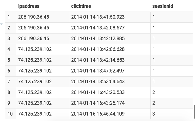
First, in subquery b, we use the LAG(col) function to calculate the time difference between current row and previous row, and if it’s more than 30 minutes, a new session is marked. Then we do a cumulative sum of the new_session field so that each session will get an incremental sequence.
1 | SELECT |
Implementation Detail
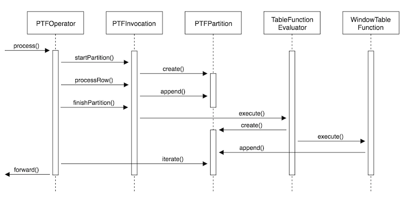
Briefly speaking, window query consists of two steps: divide records into partitions, and evaluate window functions on each of them. The partitioning process is intuitive in map-reduce paradigm, since Hadoop will take care of the shuffling and sorting. However, ordinary UDAF can only return one row for each group, but in window query, there need to be a table in, table out contract. So the community introduced Partitioned Table Function (PTF) into Hive.
PTF, as the name suggests, works on partitions, and inputs / outputs a set of table rows. The following sequence diagram lists the major classes of PTF mechanism. PTFOperator reads data from sorted source and create input partitions; WindowTableFunction manages window frames, invokes window functions (UDAF), and writes the results to output partitions.
The HIVE-896 ticket (link) contains discussions on introducing analytical window functions into Hive, and this slide (link), authored by one of the committers, explains how they implemented and merged PTF into Hive.