Pandas and Tidy Data

In the paper Tidy Data, Dr. Wickham proposed a specific form of data structure: each variable is a column, each observation is a row, and each type of observational unit is a table. He argued that with tidy data, data analysts can manipulate, model, and visualize data more easily and effectively. He lists five common data structures that are untidy, and demonstrates how to use R language to tidy them. In this article, we’ll use Python and Pandas to achieve the same tidiness.

Source code and demo data can be found on GitHub (link), and readers are supposed to have Python environment installed, preferably with Anaconda and Spyder IDE.

Column headers are values, not variable names

import pandas as pd
df = pd.read_csv('data/pew.csv')
df.head(10)

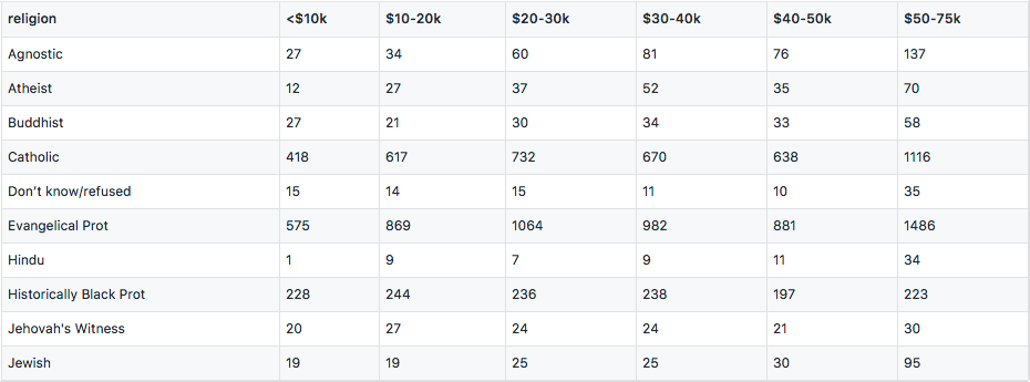
Column names “<$10k”, “$10-20k” are really income ranges that constitutes a variable. Variables are measurements of attributes, like height, weight, and in this case, income and religion. The values within the table form another variable, frequency. To make each variable a column, we do the following transformation:

df = df.set_index('religion')
df = df.stack()
df.index = df.index.rename('income', level=1)
df.name = 'frequency'
df = df.reset_index()
df.head(10)

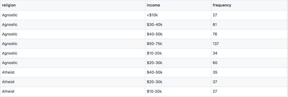
Here we use the stack / unstack feature of Pandas MultiIndex objects. stack() will use the column names to form a second level of index, then we do some proper naming and use reset_index() to flatten the table. In line 4 df is actually a Series, since Pandas will automatically convert from a single-column DataFrame.

Pandas provides another more commonly used method to do the transformation, melt(). It accepts the following arguments:

• frame: the DataFrame to manipulate.
• id_vars: columns that stay put.
• value_vars: columns that will be transformed to a variable.
• var_name: name the newly added variable column.
• value_name: name the value column.

df = pd.read_csv('data/pew.csv')
df = pd.melt(df, id_vars=['religion'], value_vars=list(df.columns)[1:],
             var_name='income', value_name='frequency')
df = df.sort_values(by='religion')
df.to_csv('data/pew-tidy.csv', index=False)
df.head(10)

This will give the same result. We’ll use melt() method a lot in the following sections.

Let’s take a look at another form of untidiness that falls in this section:

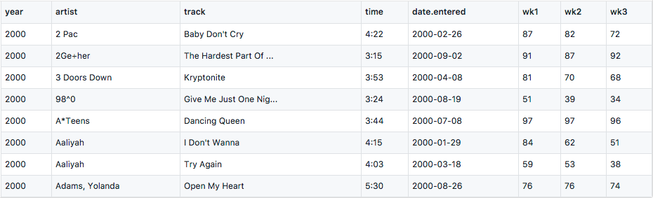
In this dataset, weekly ranks are recorded in separate columns. To answer the question “what’s the rank of ‘Dancing Queen’ in 2000-07-15”, we need to do some calculations with date.entered and the week columns. Let’s transform it into a tidy form:

df = pd.read_csv('data/billboard.csv')
df = pd.melt(df, id_vars=list(df.columns)[:5], value_vars=list(df.columns)[5:],
             var_name='week', value_name='rank')
df['week'] = df['week'].str[2:].astype(int)
df['date.entered'] = pd.to_datetime(df['date.entered']) + pd.to_timedelta((df['week'] - 1) * 7, 'd')
df = df.rename(columns={'date.entered': 'date'})
df = df.sort_values(by=['track', 'date'])
df.to_csv('data/billboard-intermediate.csv', index=False)
df.head(10)

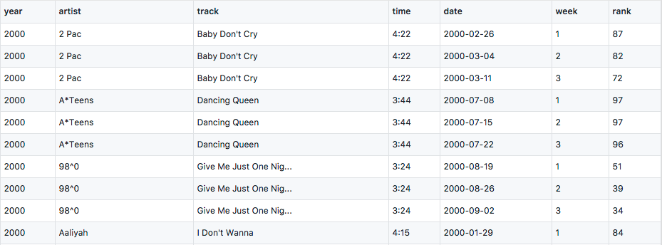
We’ve also transformed the date.entered variable into the exact date of that week. Now week becomes a single column that represents a variable. But we can see a lot of duplications in this table, like artist and track. We’ll solve this problem in the fourth section.

Multiple variables stored in one column

Storing variable values in columns is quite common because it makes the data table more compact, and easier to do analysis like cross validation, etc. The following dataset even manages to store two variables in the column, sex and age.

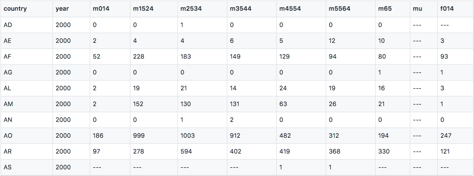
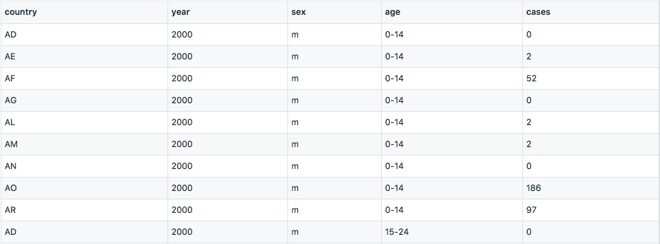
m stands for male, f for female, and age ranges are 0-14, 15-24, and so forth. To tidy it, we first melt the columns, use Pandas’ string operation to extract sex, and do a value mapping for the age ranges.

df = pd.read_csv('data/tb.csv')
df = pd.melt(df, id_vars=['country', 'year'], value_vars=list(df.columns)[2:],
             var_name='column', value_name='cases')
df = df[df['cases'] != '---']
df['cases'] = df['cases'].astype(int)
df['sex'] = df['column'].str[0]
df['age'] = df['column'].str[1:].map({
    '014': '0-14',
    '1524': '15-24',
    '2534': '25-34',
    '3544': '35-44',
    '4554': '45-54',
    '5564': '55-64',
    '65': '65+'
})
df = df[['country', 'year', 'sex', 'age', 'cases']]
df.to_csv('data/tb-tidy.csv', index=False)
df.head(10)

Variables are stored in both rows and columns

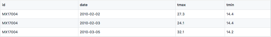
This is a temperature dataset collection by a Weather Station named MX17004. Dates are spread in columns which can be melted into one column. tmax and tmin stand for highest and lowest temperatures, and they are really variables of each observational unit, in this case, each day, so we should unstack them into different columns.

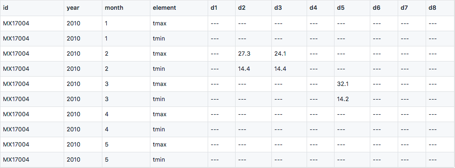
df = pd.read_csv('data/weather.csv')
df = pd.melt(df, id_vars=['id', 'year', 'month', 'element'],
             value_vars=list(df.columns)[4:],
             var_name='date', value_name='value')
df['date'] = df['date'].str[1:].astype('int')
df['date'] = df[['year', 'month', 'date']].apply(
    lambda row: '{:4d}-{:02d}-{:02d}'.format(*row),
    axis=1)
df = df.loc[df['value'] != '---', ['id', 'date', 'element', 'value']]
df = df.set_index(['id', 'date', 'element'])
df = df.unstack()
df.columns = list(df.columns.get_level_values('element'))
df = df.reset_index()
df.to_csv('data/weather-tidy.csv', index=False)
df

Multiple types in one table

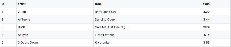
In the processed Billboard dataset, we can see duplicates of song tracks, it’s because this table actually contains two types of observational units, song tracks and weekly ranks. To tidy it, we first generate identities for each song track, i.e. id, and then separate them into different tables.

df = pd.read_csv('data/billboard-intermediate.csv')
df_track = df[['artist', 'track', 'time']].drop_duplicates()
df_track.insert(0, 'id', range(1, len(df_track) + 1))
df = pd.merge(df, df_track, on=['artist', 'track', 'time'])
df = df[['id', 'date', 'rank']]
df_track.to_csv('data/billboard-track.csv', index=False)
df.to_csv('data/billboard-rank.csv', index=False)
print(df_track, '\n\n', df)

One type in multiple tables

Datasets can be separated in two ways, by different values of an variable like year 2000, 2001, location China, Britain, or by different attributes like temperature from one sensor, humidity from another. In the first case, we can write a utility function that walks through the data directory, reads each file, and assigns the filename to a dedicated column. In the end we can combine these DataFrames with pd.concat. In the latter case, there should be some attribute that can identify the same units, like date, personal ID, etc. We can use pd.merge to join datasets by common keys.

References

• https://tomaugspurger.github.io/modern-5-tidy.html
• https://hackernoon.com/reshaping-data-in-python-fa27dda2ff77
• http://www.jeannicholashould.com/tidy-data-in-python.html